Updated
20 Oct 2025Form Number
LP2130PDF size
27 pages, 1.4 MBAbstract
The LLM Sizing Guide whitepaper provides a comprehensive framework for understanding the computational requirements of Large Language Models (LLMs). It is an essential resource for solutions architects, offering detailed insights into estimating GPU memory needs, gathering customer requirements, and optimizing system configurations. By following this guide, architects can design efficient and cost-effective systems tailored to specific customer use cases, ensuring optimal performance and resource utilization.
Change History
Changes in the October 20, 2025 update:
- Updated the formula to determine the minimum GPU memory requirement for fine-tuning/training - Rule of Thumb section
- Updated the information about Tensor Parallelism - Tensor Parallelism section
Introduction
Large Language Models (LLMs) have revolutionized the field of natural language processing, enabling applications such as text generation, sentiment analysis, and language translation. However, the computational requirements for running these models can be substantial, making it challenging for solution architects to design and configure systems that meet the needs of their customers.
To address this challenge, this LLM Sizing Guide is designed to provide you with a comprehensive understanding of how LLMs work, their computational requirements, and the key factors that impact their performance. The goal of this guide is to equip you with the knowledge and tools needed to assess customer requirements, design capable systems, and deliver successful LLM deployments quickly and accurately.
The guide, inspired from NVIDIA’s LLM Inference Sizing, will cover vital topics such as the rule of thumb for estimating GPU memory requirements for inferencing and training/fine-tuning, gathering requirements from customers, understanding benchmarks and performance metrics, and estimating total cost of ownership. By following this guide, you will be able to navigate the complex landscape of LLMs and provide their customers with optimized solutions that meet their specific needs.
Throughout this guide, we will provide practical examples, formulas, and guidelines to help solution architects estimate the computational requirements for various LLM scenarios. We will also discuss the importance of understanding customer requirements, such as model, quantization, token size, and latency requirements and how these factors impact system design and performance.
In the next section, we will introduce the "Rule of Thumb" for estimating GPU memory requirements, starting with inferencing. This will provide you with a simple and effective way to estimate the minimum GPU memory needs for running LLMs in production environments.
Rule of Thumb
The Rule of Thumb provides a simplified approach to estimating the computational requirements for running Large Language Models (LLMs). This section outlines the key factors that impact GPU memory requirements and provides formulas for quickly estimating the minimum memory needs for inferencing and fine-tuning/training.
Inferencing
Inferencing refers to the process of using a trained LLM to generate text or make predictions on new, unseen data. To estimate the minimum GPU memory requirement for inferencing, we can use the following formula:

Where:
- 𝑀model = GPU memory allocated for model, expressed in Gigabytes
- 𝑃 = Model (parameter) size in Billions
- 𝑍 = Quantization factor in Bytes (1 Byte = 8 bits) - see below
- 1.2 = Represents a 20% overhead for loading additional data into GPU memory
The quantization factor 𝑍 varies depending on the precision used:
- INT4: 𝑍 = 0.5
- FP8/INT8: 𝑍 = 1
- FP16: 𝑍 = 2
- FP32: 𝑍 = 4
For example, to estimate the minimum GPU memory requirement for running Llama 3.1 with 70 billion parameters at 16-bit quantization (FP16), we can plug in the values as follows:
𝑀 = 70 ∗ 2 ∗ 1.2 = 168 GB
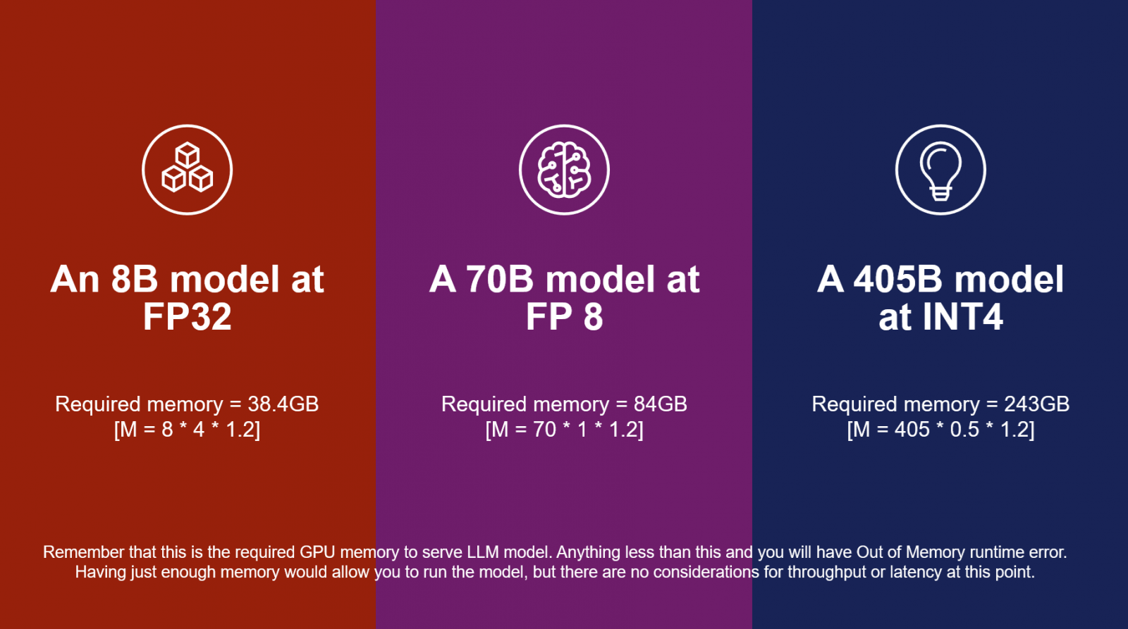
Figure 1: Example GPU Memory requirements for inferencing
This formula provides a quick and simple way to estimate the minimum GPU memory requirement for inferencing, allowing solution architects to design systems that meet the needs of their customers.
Fine-Tuning/Training
Fine-tuning or training a Large Language Model (LLM) requires considerably more computational resources than inferencing. The minimum GPU memory requirement for fine-tuning/training can be estimated using the following formula:
Total = (𝑍p + 3𝑍o + 𝑍p) bytes/parameter = 𝑃 * (2𝑍p + 3𝑍o) GB memory needed
Where:
- 𝑃 = Model (parameter) size in billions
- 𝑍p = Quantization factor in Bytes (1 Byte = 8 bits) applied to the Model Parameters to the gradients (often matches model weights precision
- 𝑍o = Quantization factor in Bytes (1 Byte = 8 bits) applied to the 3 copies of optimizer state (i.e.: at FP32 it will be 4 Bytes * 3 copies = 12)
However, this formula provides an extreme estimate, as it assumes that the full model parameters, optimizer states, and gradients are stored in memory. In practice, techniques like Low-Rank Adaptation (LoRA) and Quantized LoRA (QLoRA) can drastically reduce the memory requirements.
To give you a better idea, here are some estimated GPU memory requirements for fine-tuning LLMs using different methods and precisions:
| Method | Precision | 7B | 13B | 30B | 70B | 110B |
|---|---|---|---|---|---|---|
| Full | 16 | 67GB | 125GB | 288GB | 672GB | 1056GB |
| LoRA | 16 | 15GB | 28GB | 63GB | 146GB | 229GB |
| QLoRA | 8 | 9GB | 17GB | 38GB | 88GB | 138GB |
| QLoRA | 4 | 5GB | 9GB | 20GB | 46GB | 72GB |
As you can see, LoRA and QLoRA drastically reduce memory usage by 75-90% compared to full fine-tuning, by storing only the adapted parameters. QLoRA goes further by using 4-bit NormalFloat (NF4) to compress matrices, enabling efficient optimization on a single GPU and cutting memory needs by up to 4x.
When designing systems for fine-tuning/training LLMs, it is critical to consider the specific method and precision used, as well as the model size, to ensure that the system meets the required computational resources. By using techniques like LoRA or QLoRA, solution architects can design more efficient and cost-effective systems that meet the needs of their customers.
Gathering requirements
To accurately determine the necessary system configuration for a Large Language Model (LLM) deployment, it is important to gather specific requirements from the customer. These requirements will help estimate inference performance and ensure the system meets the desired goals.
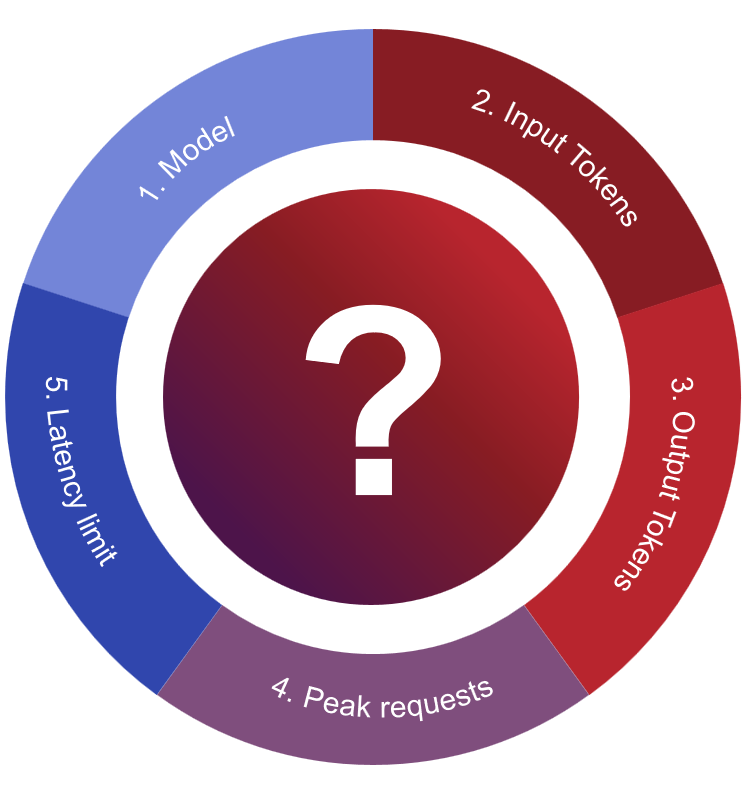
Figure 2: Gathering necessary requirements for sizing
The following five pieces of information should be collected before estimating inference performance:
- Model Selection:
Identify the LLM model intended for use in this project. The size of the model notably impacts inference performance, with larger models being slower and more expensive. Note that smaller models can have excellent quality for specific tasks while reducing inference costs. Therefore, it is recommended to explore smaller models as well. Understanding the chosen model's characteristics will help in estimating the computational resources required.
When gathering requirements for an LLM use case, it is vital to consider the input token length, which is one of the factors in determining the model's performance. The context window, defined as the sum of input and output tokens, plays a substantial role in this process. New models, such as Llama 3.1, support larger context windows of up to 128,000 tokens.
- Input Tokens:
Determine the average number of tokens in the prompt to the LLM, including:
- System prompt
- Context
- User prompt
For English language models, one token is approximately 0.75 of a word. Including system prompts and context in the token count ensures that the entire input sequence is considered when estimating performance.
To accurately calculate the input token count, include all elements that contribute to it, such as system prompts (custom instructions), retrieved documents (in Retrieval Augmented Generation pipelines), and chat history (previous conversation exchanges). Each of these components counts towards the maximum budget of tokens that can be passed into the model.
Large input length can impact inference performance, as words are converted to embeddings and KV cache grows quadratically. Applications like RAG pipelines may require larger input lengths, resulting in increased first-token latency due to the substantial amount of data being processed.
We will delve deeper into tokens and their impact on latencies later in this paper, exploring how they affect the performance of LLMs and what considerations are necessary for optimal model operation.
- Output Tokens:
Establish the average number of tokens in the LLM output. This is necessary because generating more tokens requires more computational resources and time. Understanding the expected output size will help in designing a system that can handle the required throughput without compromising on latency or quality.
- Average Requests per Second (RPS):
To ensure optimal performance and efficient resource utilization, determine the peak number of requests the system should process per second. When sizing for on-premises deployments, it is vital to base calculations on peak usage, rather than average usage.
To account for variability in request patterns, we use the 95th percentile of the Poisson PPF (point probability function) of average RPS (requests per second). This approach helps to identify the maximum expected load, allowing us to design a system that can handle peak demands without being underutilized during non-peak periods.
The process involves obtaining the average request rate from the customer and calculating the peak request rate using the 95th percentile of the Poisson distribution. This method provides a more accurate representation of the system's requirements, as it considers the natural variability in request patterns. It is particularly important to note that if the system is not running at peak capacity, the effective cost per token can increase considerably.
- Latency Requirements:
Understand the customer's latency goals and limits, including:
- First-token latency: The time it takes for the model to generate the first token of the response.
- Last-token latency: The total time it takes for the model to generate the entire response.
Latency is a critical factor in many applications, as high latency can negatively impact user experience. Constraining to a lower first-token latency (TTFT) would drastically hamper throughput, meaning that the system's ability to process multiple requests simultaneously would be compromised. Therefore, it's essential to strike a balance between latency and throughput based on the customer's specific requirements.
These requirements are crucial for estimating inference performance, sizing the system, and ensuring it meets the customer's expectations. By gathering this information, you'll be able to better understand the customer's needs and design an appropriate system configuration that balances performance, cost, and quality. In the next sections, we will delve deeper into some of these requirements and explore how they impact LLM deployment.
Sizing LLMs for Inferencing based on requirements
Now that we have gathered the requirements and understood the use-case the customer wants, we can provide an estimate for the amount of VRAM (GPU memory) required for system sizing. Before we provide a quick formula for calculation, there’s one important metric to consider when it comes to LLM Sizing which is Key-Value (KV) cache that affects our calculation.
KV Caching: A Crucial Component for Efficient Inference in Large Language Models
KV caching is an optimization technique used in large language models (LLMs) to store key and value tensors from past tokens. This method reduces computational overhead by avoiding redundant calculations at each generation step, thereby improving efficiency both computationally and in terms of memory usage.
Understanding Factors Affecting KV Cache Size
The KV cache depends on the use case, the scale of the solution, and the model proposed to be used. Different models have different architectures which affect the KV cache size. These parameters collectively define the memory requirements for storing the key and value tensors:
- Concurrent Users (Batch Size): The number of samples processed simultaneously entails parallel tracking of individual KV caches. Larger batches increase the memory required for the KV cache.
- Sequence Length: The total context window of the model comprising of all input tokens and generated output tokens. Longer sequences mean more tokens stored, increasing KV cache size.
- Number of Attention Heads: Multi-head attention (MHA) mechanisms split the input into multiple representations. More heads can lead to a larger KV cache. However, latest architectural innovation in models attempt to reduce those.
- Hidden Dimension Per Head: The dimensionality of each head's output vectors. Higher dimensions increase the memory footprint. Sometimes model providers specify model dimensions directly (Dmodel) which is just total number of dimensions in whole model (Nheads X Dhead)
- Precision (Bytes): The data type used for storage, such as FP16 or FP32, affects memory usage. Lower precision uses fewer bytes. Also known as the Quantization factor.
Optimizing KV cache
Multi-Head Attention (MHA) is a fundamental mechanism in transformer models, where multiple attention heads are used to capture different aspects of the input data. Each head independently computes attention scores, allowing the model to focus on various parts of the input simultaneously. This parallel processing enhances the model's ability to understand complex patterns and relationships within the data. However, MHA comes with a significant limitation: the size of the Key-Value (KV) cache. As the number of attention heads increases, the KV cache size grows proportionally, leading to substantial memory overhead, especially for long sequences. This can hinder the efficiency and scalability of large language models (LLMs), as the KV cache can become larger than the model's parameter memory.
Recent innovations like Multi-Query Attention (MQA) and Grouped Query Attention (GQA) offer promising solutions to reduce KV cache size. MQA simplifies the attention mechanism by using a single set of keys and values for all query heads, significantly reducing the memory bandwidth required. This approach decreases the KV cache size by a factor of the number of heads. But having a single set of KV may not provide the required complexity. GQA treads the balance by grouping query heads, allowing each group to share a single set of keys and values. It introduces a grouping factor (g) that represents the number of query heads in each group which can achieve reductions in KV cache size. By leveraging these techniques, LLMs can maintain high performance with a more manageable memory footprint, making them more efficient and scalable for various applications.
Calculating KV cache
Now that we understood all the factors affecting KV cache size, we can estimate the memory requirements by using a formula given below:

Where:
- 𝑀KV = GPU memory allocated for KV cache expressed in bytes
- 2 = Factor since we store two vectors (key and value) each
- Cusers= Number of concurrent users/requests a.k.a Batch Size
- Tseq= Average context token sequence length per user
- Llayers= Number of layers in transformer
- Nattn_heads = number of attention heads
- g = Grouping factor (g is 1 for MHA, g is NKV heads for MQA, and in between for GQA)
- Dhead= Dimension of each head
- 𝑍bytes = Quantization factor in Bytes (1 Byte = 8 bits)
Information about open-source models factors are available from the model provider. Some providers give the value of NKV_heads which considers the grouping factor directly

Example sizing to calculate VRAM requirement
With an example sizing and calculating the required memory will give us the idea of what GPUs may be needed for a particular task.
Now let’s consider an organization who wants to use a chatbot with internal sensitive documents. After gathering the requirements, we understand that they want to use a Llama 3.3 70B model at FP16 precision for 100 concurrent users with an average context of 8000 tokens (7000 input and 1000 output). Provided by Meta, the Llama model has 80 layers, each having 64 attention heads, 8 KV heads, and 128 head dimensions in GQA format.
Using the gathered information, we can calculate the required model memory (and account for overhead) as follows:

Mmodel = 70 x 2 x 1.2
Mmodel = 168 GB
And the KV cache calculation is as follows:

MKV = 2 x 100 x 8000 x 80 x 8 x 128 x 2
MKV = 262144000000 bytes
MKV = 262.144 GB
Hence,

Mtotal = 168 GB + 262.144 GB
Mtotal = 430.144 GB
As we can see, depending on the scale of the solution, the KV cache memory requirement can be larger than model itself! Therefore, it is vital to include all components during the sizing calculation.
In conclusion, accurately sizing LLMs for inferencing requires a comprehensive understanding of both the model's architecture and the specific use-case requirements. By considering factors such as the number of concurrent users, sequence length, number of attention heads, hidden dimensions per head, and precision, we can estimate the VRAM needed for efficient operation. Innovations like MQA and GQA significantly optimize KV cache size, making it feasible to deploy large models without prohibitive memory overhead. This holistic approach ensures that the system is both performant and scalable, meeting the demands of modern applications while maintaining efficiency.
Technical Dive: Understanding LLMs
In this section, we will explore the intricate workings of Large Language Models (LLMs) by diving into their technical aspects. We will investigate stages of LLM execution, understand key measurement metrics, and look at techniques that speed up inferencing.
In this section:
Two Stages of LLM Execution: Prefill vs Decoding
Large Language Models (LLMs) are complex systems that involve multiple stages of processing to generate human-like text responses. Understanding these stages is helpful for optimizing performance, reducing latency, and improving overall user experience. In this section, we will delve into the two primary stages of LLM execution: Prefill and Decoding.
Prefill Stage
The Prefill stage refers to the time it takes for an LLM to process a user's input prompt and generate the first output token, which is approximately equivalent to a word. This stage encompasses the following steps:
- Loading the user prompt: The user's input is received and loaded into the system.
- Populating KV-cache: During this stage, the LLM populates its Key-Value (KV) cache with information from the input tokens. This cache is used to store and retrieve relevant context-specific data.
- Request reception to first token: The time it takes for the LLM to process the input prompt and generate the first output token.
The Prefill stage is primarily compute-bound, meaning that its performance is largely dependent on the computational resources available. The time it takes to complete this stage depends only on the number of input tokens, making it a predictable and consistent process.
Decoding Stage
The Decoding stage, also known as generation or expansion, is where the LLM generates response tokens one by one, building upon the initial output token produced during the Prefill stage. This stage involves:
- Inter-token latency: The time it takes to generate each subsequent token after the first one.
- Token-by-token generation: The LLM generates response tokens word by word, using the context and information gathered during the Prefill stage.
- Dependency on input and output tokens: The inter-token latency depends on both the number of input tokens and the number of output tokens being generated.
In contrast to the Prefill stage, Decoding is typically memory-bound, meaning that its performance is heavily influenced by the availability of memory resources. As the LLM generates more tokens, it requires more memory to store and manage the growing context, which can lead to increased latency.
LLM Inference Measurement Metrics
When evaluating the performance of Large Language Models (LLMs), several key metrics are used to measure inference speed. These include:
- Time to First Token (TTFT): The time it takes to process the input and generate the first token.
- Inter-token Latency (ITL): The time it takes to generate each subsequent token after the first one, also known as Time Per Output Token (TPOT).
- End-to-End Latency (E2E): The total time it takes to process a prompt and generate all the tokens, from input to output.
These metrics provide insights into the model's performance, helping to identify bottlenecks and optimize inference speed.
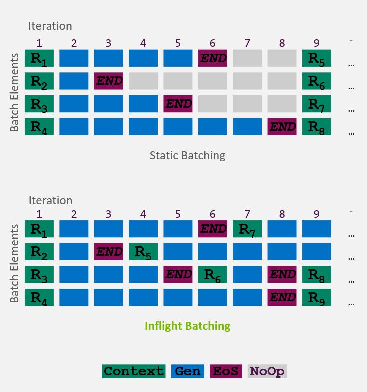
Inflight batching
Inflight batching (IFB) is a specialized technique used during Large Language Model (LLM) inference to strike a balance between GPU memory and compute utilization, ultimately reducing latency. This method is particularly effective in auto-regressive inference, where the LLM generates tokens sequentially, relying on previously generated tokens to produce the next ones.
IFB allows sequences at various stages (both prefill and decoding) to be processed within the same batch without waiting for all requests to complete before introducing new ones. This approach offers several key benefits:
- Constant Batch Size: IFB enables a nearly constant batch size for each token generation, leading to higher GPU utilization.
- Quicker Execution Starts: New requests can begin execution more quickly when slots become available, as the scheduler only waits for the next token's generation rather than the completion of current requests.
TensorRT-LLM incorporates custom Inflight Batching to optimize GPU utilization during LLM serving. This feature:
- Replaces completed requests in the batch.
- Evicts requests after the End-of-Sequence (EoS) marker and inserts new requests.
- Improves throughput, time to first token, and overall GPU utilization.
Moreover, IFB is seamlessly integrated into the TensorRT-LLM Triton backend and can be managed through the TensorRT-LLM Batch Manager. When combined with other techniques such as balancing memory-bound and compute-bound operations, chunked decoding, speculative decoding, and sparsity, IFB enhances the throughput of LLMs, making it an indispensable tool for efficient LLM inference.
Tensor Parallelism
Tensor Parallelism (TP) is one of the techniques utilized in Large Language Model (LLM) inference to distribute the computational load across multiple GPUs. This method involves splitting one model (and the relative KV Cache) across several GPUs, which relies heavily on efficient data exchange between these GPUs. TP is particularly beneficial for larger models where the memory requirements exceed the capacity of a single GPU. It is also one of the most efficient parallelization strategy since it provides an optiomal tradeoff in terms of latency vs throughput.
Key characteristics of Tensor Parallelism:
- Lower Latency but Lower Throughput: While TP can reduce latency by parallelizing computations, it may also lead to lower overall throughput due to the overhead associated with inter-GPU communication.
- Requirement for Bigger Models: For larger models like LLaMa-70B, a tensor parallelism of at least 2 (TP >= 2) is required. This ensures that the model can be adequately split across multiple GPUs to fit within the available memory and computational resources.
- Recommendation for NVLink-enabled Servers: When TP exceeds 2, NVIDIA strongly recommends using NVLink-enabled servers for inference. NVLink provides a high-bandwidth, low-latency interconnect that significantly improves data transfer between GPUs compared to traditional PCIe connections.
Understanding benchmarks
Benchmarks are central in sizing and choosing an ideal configuration for customers, as they evaluate tradeoffs between key metrics like throughput, latency, and request rate. Understanding these benchmarks helps determine the optimal configuration for large language model (LLM) inference, allowing informed decisions about hardware and software requirements.
In this section:
Throughput vs Latency
In the context of LLM inference, achieving a balance between throughput and latency is critical. Throughput refers to the number of requests that can be processed per unit time, while latency is the time taken to process a single request from start to finish.
The Tradeoff:
Introducing latency limits can decrease available throughput. Conversely, relaxing latency constraints can lead to much higher throughput. Understanding customer use cases provides estimates of input tokens, output tokens, and average requests per unit time, allowing for the proposal of specific hardware that matches required throughput while maintaining necessary latency.
Combining multiple requests to increase throughput can introduce delays, increasing latency for individual requests. LLM inference involves two phases - prefill (high latency, benefits from parallel processing) and decode (lower latency, lower compute utilization).
Practical Implications:
- High Throughput: Ideal for large-scale deployments with high request volumes.
- Low Latency: Crucial for real-time response applications, such as conversational AI or interactive systems.
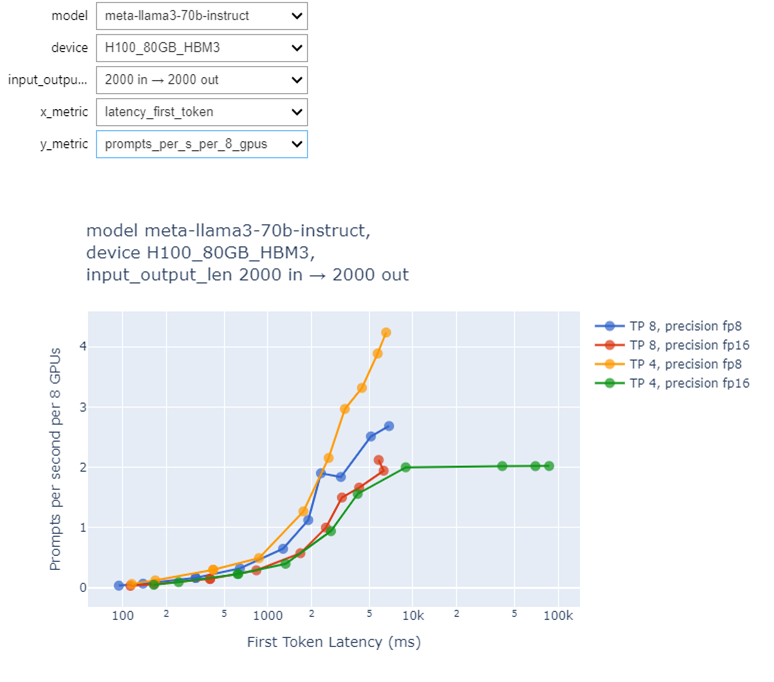
Figure 4: Throughput vs First Token Latency graph for Llama 3 70B model with 2000 input and 2000 output tokens
By understanding and managing the throughput-latency tradeoff, LLM inference systems can be optimized to meet specific application requirements. For custom benchmarking, tools like GenAI-Perf by NVIDIA can provide valuable insights into a particular model's performance on a system.
To learn how to interpret the benchmark graphs, see the topic at the end of this document, Additional Information - Reading the graphs for sizing.
Understanding Max Batch Size, Concurrency, Request Rate, and Throughput
It can get a little confusing handling all the jargons, so let's break down each concept to clarify their relationships and importance in system evaluation.
- Max Batch Size
- Batch Size and Concurrency
- Concurrency and Request Rate as a Result Metric
- Concurrency and Request Rate as an Input Parameter
- Recommendations
Max Batch Size
The max_batch_size parameter has two roles: one during engine build and another at runtime.
- Engine Build: This setting ensures that the resulting system, with its capacity for a certain batch size, fits within the available memory. It's essentially about capacity planning to prevent memory issues during execution.
- Runtime: This setting determines how many requests can be batched together before being processed. The runtime max_batch_size must be less than or equal to the build-time max_batch_size. The actual batching of requests in real scenarios is influenced by this parameter, directly affecting efficiency and performance.
Batch Size and Concurrency
- Concurrency (C) < Max Batch Size (MBS): When the number of concurrent requests is less than the maximum batch size, the engine typically processes batches with a size equal to the concurrency level. This means there are free slots available in each batch, as not all potential positions in the batch are filled.
- Concurrency (C) >= Max Batch Size (MBS): If concurrency equals or exceeds the max batch size, then the batches are usually full, processing at maximum capacity. The queue for new requests will start to grow, with an average size of C - MBS, as incoming requests wait for previous batches to finish.
Concurrency and Request Rate as a Result Metric
To gauge system performance comprehensively, consider:
- Throughput: The number of requests the system can process per unit time.
- End-to-end Latency: The total time taken for a request to be processed from start to finish.
- Concurrency: The number of requests that can be handled simultaneously.
A system with high concurrency and high latency might achieve the same throughput as one with lower concurrency but lower latency. However, the latter is more efficient because it responds faster to individual requests.
Therefore, using "requests per minute" (or a similar time-based metric) as the primary measure for sizing systems and discussing performance with stakeholders provides a balanced view of system capacity. It helps factor in both concurrency and latency requirements, offering a clearer picture of what the system can handle efficiently.
Concurrency and Request Rate as an Input Parameter
For accurate speed measurements (throughput), it's indispensable to maintain a constant engine batch size from one processing cycle to another.
- Using Concurrency as an Input: This approach ensures that the batch size remains consistent, providing reliable measurements.
- Setting a Request Rate as Input Parameter: This can be problematic because if the request rate exceeds the system's throughput, the queue will continuously grow, increasing latency. Conversely, setting a request rate below the system's throughput means not all available slots are utilized, leading to underperformance.
Recommendations
- Use Concurrency with Token Sizes as Input Metrics: This allows for controlled experiments that can stress the system to its limits or measure its responsiveness under lighter loads.
- Use Request Rate as a Result Metric: It provides insight into how many requests the system can actually process within a given timeframe, reflecting both its capacity and efficiency.
By controlling these parameters and focusing on the right metrics, enterprises can design more efficient systems that balance throughput, latency, and resource utilization effectively.
Total Cost of Ownership: Cloud vs On-prem
Deploying Large Language Model (LLM) inferencing is becoming essential for modern businesses. There are two main options: cloud-based and on-premise. We will explore the benefits and limitations of each option to help you make an informed decision.
In this section:
Cloud-Based Deployment
Cloud-based deployment offers a "pay-as-you-go" model, where you only pay for the resources used. However, there are some drawbacks to consider:
- Data Security: Unless an enterprise-grade license is purchased, your data may be used to train future models, potentially leading to data leakage.
- Price Uncertainty: Prices are subject to change, and you have less control over the model, which may not support fine-tuning or customizations.
- Limited Control: You have limited control over the latency and throughput of the prompts.
The cost of cloud-based deployment is typically calculated based on input and output tokens, with a fixed price per token. For example, one million input tokens may cost $15, while a million output tokens cost $60. To estimate the cost, you can use a calculator that considers the number of input and output tokens.
On-Premise Deployment
On-premise deployment requires a substantial upfront investment but offers several benefits:
- Complete Control: You have complete control over the system, allowing for changes as needed.
- Cost-Effective: With a fixed utilization near capacity, on-premise deployment can be cost-effective in the long run.
- Security: Your data is secure, and you have full control over the system.
The costs associated with on-premise deployment include:
- GPU Server Purchase: The price of purchasing a GPU server, which varies depending on the hardware and type of system.
- Datacenter Costs: Costs related to electricity, renting space, staff, and other expenses.
- License Fees: An annual license fee for any additional services e.g., NVAIE
To find the cost per 1M prompts (calls):

Simplifying,

where
- Z = Cost per 1M prompts
- C = Total On Prem Cost averaged over a year
- X = Prompts per second (throughput) on system
Comparison of Cloud and On-Premise Deployment
To make a fair comparison between cloud and on-premise deployment, we assume that:
- The models deployed on both platforms are equivalent in quality.
- The latency and throughput achieved on both platforms are similar.
We can compare the on-prem costs per 1M prompts to on-cloud costs per 1M prompts to get a fair comparison. We could even find out per input token and output token cost for on-prem.
Cost recap
In conclusion, both cloud-based and on-premise deployment options have their benefits and limitations. Cloud-based deployment offers a flexible and scalable solution but may compromise on data security and control. On-premise deployment provides complete control and security but requires an upfront investment. In long-term, a break-even point is reached where the on-premise deployment makes financial sense than on-cloud instances.
Recommendation
When deciding between cloud-based and on-premise deployment, consider the following:
- Data security: If it's your top priority, on-premise deployment is better.
- Scalability: If you need to scale quickly, cloud-based deployment might be more suitable.
- Budget: If budget is a concern, on-premise deployment can be cost-effective in the long run.
Ultimately, the decision depends on your specific needs and priorities.
Conclusion
In conclusion, accurately estimating performance and computational requirements is crucial when designing systems for Large Language Model (LLM) deployment. To achieve this, gather specific requirements from customers, including model selection, input token length, quantization, and latency needs. The provided formulas and guidelines, such as the "Rule of Thumb" for estimating GPU memory requirements, serve as valuable tools for solution architects to quickly assess and design capable systems that meet customer demands.
By considering key factors like model size, precision, and quantization, you can optimize system configurations to balance performance and cost. Additionally, techniques like Low-Rank Adaptation (LoRA) and Quantized LoRA (QLoRA) can radically reduce memory requirements during fine-tuning and training, enabling more efficient and cost-effective solutions.
This LLM Inference Sizing Guide empowers with the knowledge and expertise needed to navigate the complex landscape of LLMs, deliver successful deployments, and provide tailored solutions that meet the unique needs of their customers. By following these guidelines and best practices, you can ensure optimal performance, reduce costs, and drive business success in the rapidly evolving field of natural language processing.
Additional Information - Reading the graphs for sizing
A graph based on the benchmark data from NVIDIA NIMs looks like this:
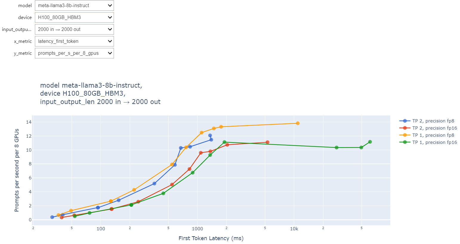
Figure 5: Sample Throughput vs First Token Latency graph for Llama 3 8B model with 2000 input and 2000 output tokens
The interactive graphs allow you to select the models, devices, input + output token combination, X-axis metric and Y-axis result. For X-axis we could have input parameters like TTFT, TTLT, or ITL for tokens. For Y-axis we have output parameters like prompts per sec per system or out_tokens per sec per system or per GPU instance.
An example sizing:
A customer wants a 2000 in, 2000 out token with llama3 8B model and wants TTFT under 1 sec. Using the constraints we find a point on the graph left of 1 sec TTFT (FTL), it would look like this:
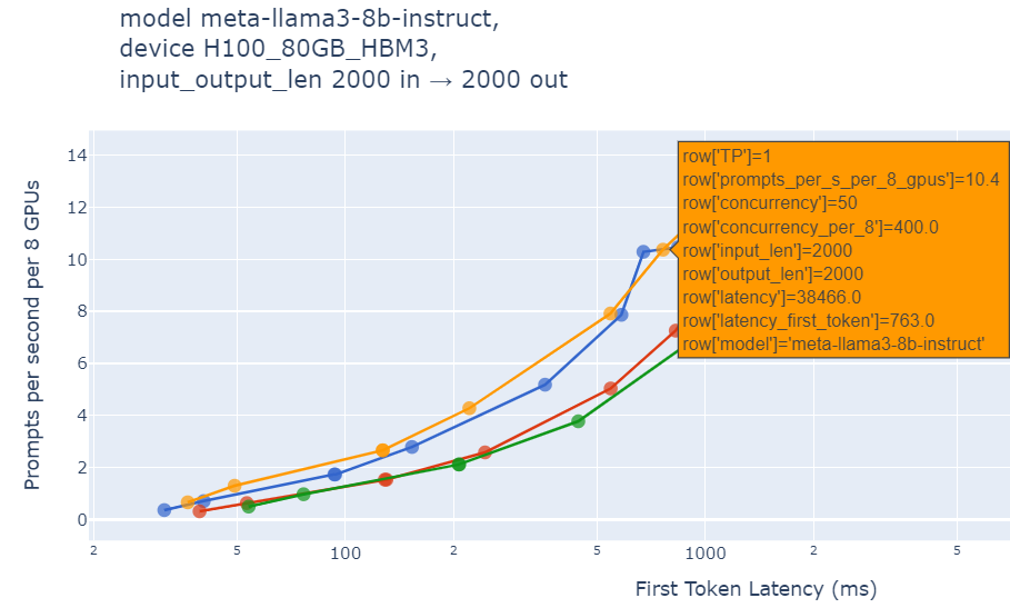
Figure 6: Choosing FTL under 1 second for Llama 3 8B model with 2000 input and 2000 output tokens
This tells you that a single 8xH100 system would be able to handle up to 400 concurrent (peak) users when using TRT-LLM. However, we see that this has the total latency over 38 seconds. If we want a lower total latency (let’s say under 20 secs), we will have to sacrifice the throughput, reforming X-axis as total latency (TTLT), we have:
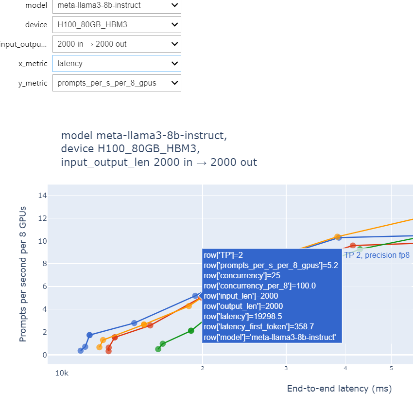
Figure 7: Choosing E2E under 20 seconds for Llama 3 8B model with 2000 input and 2000 output tokens
Here we have a point with 100 concurrent users with 358ms TTFT and under 20s TTLT. As we see, setting latency constraints heavily affects the throughput and max concurrency.
To run benchmarks on your own system, refer NVIDIA’s NIM for LLM Benchmarking Guide to use GenAI-Perf to get LLM metrics.
Authors
Sachin Gopal Wani is a Staff Data Scientist at Lenovo, working on end-to-end Machine Learning (ML) applications for varying customers. He has published articles on the sizing guide and provides sizing information for customers. Sachin holds extensive experience in AI solutions including LLMs, and Computer Vision. He graduated from Rtugers University as a gold medalist specializing in ML and has secured the J.N. Tata Scholarship.
David Ellison is the Chief Data Scientist for Lenovo ISG. Through Lenovo’s US and European AI Discover Centers, he leads a team that uses cutting-edge AI techniques to deliver solutions for external customers while internally supporting the overall AI strategy for the Worldwide Infrastructure Solutions Group. Before joining Lenovo, he ran an international scientific analysis and equipment company and worked as a Data Scientist for the US Postal Service. Previous to that, he received a PhD in Biomedical Engineering from Johns Hopkins University. He has numerous publications in top tier journals including two in the Proceedings of the National Academy of the Sciences.
Valerio Rizzo is the EMEA AI Technical Leader for Lenovo AI Advanced Solutions. He leads AI technical R&D initiatives and the deployment of advanced AI solutions across global enterprise environments, supporting both customer-facing innovation consultancy and internal enablement. With deep expertise in neuroscience and artificial intelligence, he brings a rigorous scientific approach to AI strategy and implementation. He collaborates closely with cross-functional teams to align AI capabilities with organizational goals, while also mentoring emerging talent in the field. Valerio holds a PhD in Neuroscience and has authored and contributed to scientific research through multiple publications in international peer-reviewed journals.
Trademarks
Lenovo and the Lenovo logo are trademarks or registered trademarks of Lenovo in the United States, other countries, or both. A current list of Lenovo trademarks is available on the Web at https://www.lenovo.com/us/en/legal/copytrade/.
The following terms are trademarks of Lenovo in the United States, other countries, or both:
Lenovo®
Other company, product, or service names may be trademarks or service marks of others.
Configure and Buy
Full Change History
Changes in the October 20, 2025 update:
- Updated the formula to determine the minimum GPU memory requirement for fine-tuning/training - Rule of Thumb section
- Updated the information about Tensor Parallelism - Tensor Parallelism section
Changes in the April 24, 2025 update:
- Added new section Sizing LLMs for Inferencing based on requirements which includes an example sizing
- Changed notation in formula to account for different memory expressions by model and KV cache
First published: January 24, 2025
Course Detail
Employees Only Content
The content in this document with a is only visible to employees who are logged in. Logon using your Lenovo ITcode and password via Lenovo single-signon (SSO).
The author of the document has determined that this content is classified as Lenovo Internal and should not be normally be made available to people who are not employees or contractors. This includes partners, customers, and competitors. The reasons may vary and you should reach out to the authors of the document for clarification, if needed. Be cautious about sharing this content with others as it may contain sensitive information.
Any visitor to the Lenovo Press web site who is not logged on will not be able to see this employee-only content. This content is excluded from search engine indexes and will not appear in any search results.
For all users, including logged-in employees, this employee-only content does not appear in the PDF version of this document.
This functionality is cookie based. The web site will normally remember your login state between browser sessions, however, if you clear cookies at the end of a session or work in an Incognito/Private browser window, then you will need to log in each time.
If you have any questions about this feature of the Lenovo Press web, please email David Watts at dwatts@lenovo.com.

